Simulate, Map, and Visualize LCRs: a synthetic example

This pipeline generates a FASTA file containing Low-Complexity Region (LCR) sequences, followed by its LCR mapping and visualization. To perform this pipeline, AlcoR and the following Bash script must run

#!/bin/bash
#
# This code creates a simple repetitive sequence:
#
echo ">repetitive dna" > repetitive.fa;
for((x=1;x<=100;++x));
  do
  echo "ACGTACGTACGTACGTACGTACGTACGTACGTACGTACGTACGTACGTACGTACGTACGTACGT" >> repetitive.fa;
  done
# 
# This code simulates a sequence containig LCRs in several parts:
#
AlcoR simulation -rs 2000:0:1:0:0:0 -fs 1:2000:1:3:0:0:0:repetitive.fa \
-rs 2000:0:11:0:0:0 -fs 1:2000:1:3:0:0:0:repetitive.fa -rs 2000:0:21:0:0:0 \
-rs 2000:0:17:0:0:0 -rs 2000:0:27:0:0:0 -rs 2000:0:17:0:0:0 -rs 2000:0:31:0:0:0 \
-rs 2000:0:47:0:0:0 -rs 2000:0:37:0:0:0 -rs 2000:0:55:0:0:0 -rs 2000:0:67:0:0:0 \
-rs 2000:0:17:0:0:0 -rs 2000:0:71:0:0:0 > example.fasta;
#
# This code maps the LCRs:
#
AlcoR mapper -v -w 10 --dna -m 11:50:0:1:0:0.9/0:0:0 example.fasta > LCRs.csv
#
# This code creates an image depicting the LCRs:
#
AlcoR visual -v -o map.svf LCRs.csv
#

This code will generate the following image with the LCRs for the simulated sequence characterized by the green color

Herpesvirus genomes comparative LCR Maps

This pipeline assumes that there are 9 herpesviruses genomes in each FASTA respective file with the names declared at the GENOMES array. Two types of LCRs are present: the local (within 5k symbols) and the distant. To compute the visual LCR maps without exploring the similarity between genomes, the following Bash script needs to run

#!/bin/bash
#
THRESHOLD=" 1.2 ";
#
declare -a GENOMES=("HSV-1" "HSV-2" "VZV" "EBV" "HCMV" "HHV6A" "HHV6B" "HHV7" "KSHV");
for GENOME in "${GENOMES[@]}"
  do
  AlcoR mapper -v --hide --color 100 --threshold $THRESHOLD --ignore 50 --dna -w 50 -m 13:50:0:1:10:0.9/3:10:0.9 $GENOME.fa > $GENOME-d.txt
  AlcoR mapper -v --no-size --hide --threshold $THRESHOLD --color 1 \
  --ignore 50 --dna -w 50 -m 13:50:5000:1:10:0.9/3:10:0.9 $GENOME.fa > $GENOME-l.txt
  cat $GENOME-d.txt $GENOME-l.txt > $GENOME.txt;
  done
AlcoR visual -o mapv.svg --strict-corner -s 10 -w 10 -e 0 --border-color cccccc \
HSV-1.txt:HSV-2.txt:VZV.txt:EBV.txt:HCMV.txt:HHV6A.txt:HHV6B.txt:HHV7.txt:KSHV.txt
#

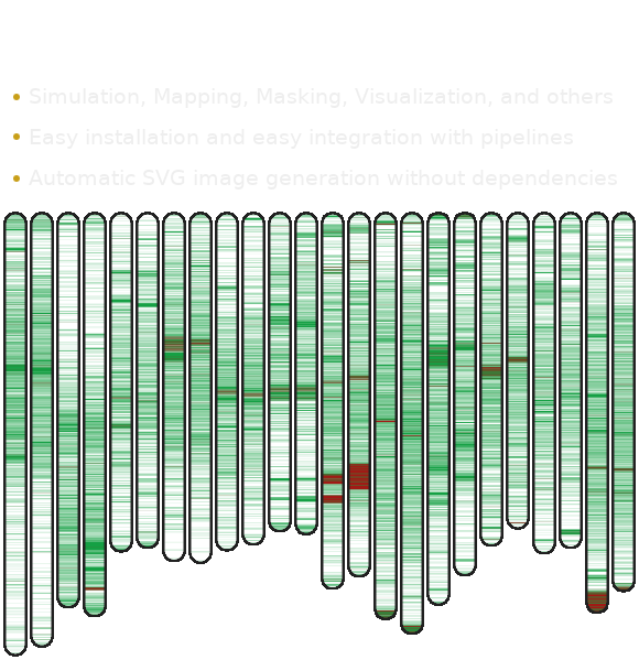
Whole-genome LCR Maps

This pipeline assumes that there are 18 chromosome sequences of the Cassava genome in the H1.fa file (multi-FASTA format). These sequence are available at the repository. The LCR are computed taking into consideration similarity between chromosomes using the following Bash script

#!/bin/bash
#
THRESHOLD=" 0.5 ";
#
AlcoR mapper -v --hide --threshold $THRESHOLD --ignore 1000 --dna -w 5000 -m 14:50:0:1:10:0.9/3:10:0.9 \
-m 13:50:5000:1:10:0.9/3:10:0.9 --renormalize --prefix W H1.fa
AlcoR visual -v -o map.svg -s 6 -w 18 -e 0 \
W1.txt:W2.txt:W3.txt:W4.txt:W5.txt:W6.txt:W7.txt:W8.txt:W9.txt:W10.txt:W11.txt:W12.txt:W13.txt:W14.txt:W15.txt:W16.txt:W17.txt:W18.txt
#

This code will generate the following image with the LCRs for each Cassava chromosome

Masking LCR sequences

This pipeline assumes that there are 18 chromosome sequences of the Cassava genome in the H1.fa file (multi-FASTA format). These sequence are available at the repository. The genome is masked into masked-H1.fa taking into consideration the similarity between chromosomes. It will ignore regions lowe than 20 symbols. The following Bash script must run

#!/bin/bash
#
THRESHOLD=" 0.5 ";
#
AlcoR mapper -v --hide --threshold $THRESHOLD --ignore 20 --dna -w 10 -m 14:50:0:1:10:0.9/3:10:0.9 \
-m 13:50:5000:1:10:0.9/3:10:0.9 -k -o masked-H1.fa --renormalize --prefix W H1.fa
#

The output are multiple FASTA files as many as the number of FASTA headers with prefix W (example: W1.txt, W2.txt, ...) and where the low complexity regions appear in lower case symbols.